Impulse, Reflection, Decay: Why Acoustic Engineers Still Trust the Time Domain Over Frequency Specs

A loudspeaker manufacturer publishes a frequency response curve that traces a remarkably flat line from 40 Hz to 20 kHz. A room acoustic consultant presents an equalization plot showing minimal deviation across the audible band. On paper, both look authoritative. In practice, neither tells an engineer how sound actually propagates through space and time—and that omission has consequences that range from listener fatigue in a corporate conference room to catastrophic intelligibility failure in a performing arts venue.

Impulse response measurement addresses precisely this gap. It is, at its core, a time-domain technique: inject a known signal into a system, capture the output, and examine the relationship between the two across every moment following the stimulus. What emerges is not a curve describing average energy at each frequency but a full temporal portrait of how sound arrives, reflects, scatters, and eventually dissipates. For acoustic engineers working on concert halls, recording studios, broadcast facilities, and home theater installations across the United States, that portrait remains indispensable.

From Pistol Shots to Swept Sines: A Brief History

Early practitioners of room acoustics had limited options. Wallace Clement Sabine, working at Harvard in the late 1890s, estimated reverberation times by listening. Decades later, engineers fired blank pistols or burst balloons and recorded the decay on chart paper. These methods produced usable data for gross reverberation estimates but offered poor resolution and were vulnerable to ambient noise contamination.

The introduction of maximum-length sequence (MLS) signals in the 1970s and 1980s represented a significant step forward. MLS stimuli are pseudorandom binary sequences with flat power spectra; by cross-correlating the system output against the known sequence, an engineer can extract an impulse response with high signal-to-noise ratio even in moderately noisy environments. The technique became a staple in research laboratories and, later, in commercial measurement software.

Today, the swept-sine method—sometimes called the exponential sine sweep or chirp technique—has largely supplanted MLS for room and loudspeaker measurement. Developed and formalized by Angelo Farina in the early 2000s, the approach drives the device under test with a sine wave whose frequency increases exponentially from the bottom to the top of the band of interest. The captured output is deconvolved with a time-reversed version of the sweep, yielding not only the linear impulse response but also a series of harmonic distortion impulse responses displaced in time. This separation of linear behavior from nonlinear artifacts makes the swept-sine approach particularly powerful for loudspeaker characterization, where driver distortion can otherwise contaminate the measurement.

What Frequency Specs Cannot Tell You

The persistence of frequency-domain thinking in acoustic specification is understandable. Frequency response is intuitive, visually compact, and easy to compare across products. The problem is that it integrates over time in a way that destroys precisely the information an engineer needs to understand subjective performance.

Consider two loudspeakers with nominally identical frequency response curves. One achieves its measured response through clean, direct radiation; the other produces the same averaged energy through a combination of direct sound and strong early reflections from its cabinet edges. A listener in a critical listening environment will perceive these two designs very differently—the second will sound colored and spatially blurred—yet the frequency plots may be indistinguishable.

The impulse response separates these cases immediately. A cumulative spectral decay (CSD) waterfall plot, derived from the impulse response, reveals resonances that ring long after the stimulus has ceased. A simple time-windowed gate isolates the direct sound from reflections. The engineer sees not just what energy is present but when it arrives and how long it persists.

Building a Competent Measurement Rig

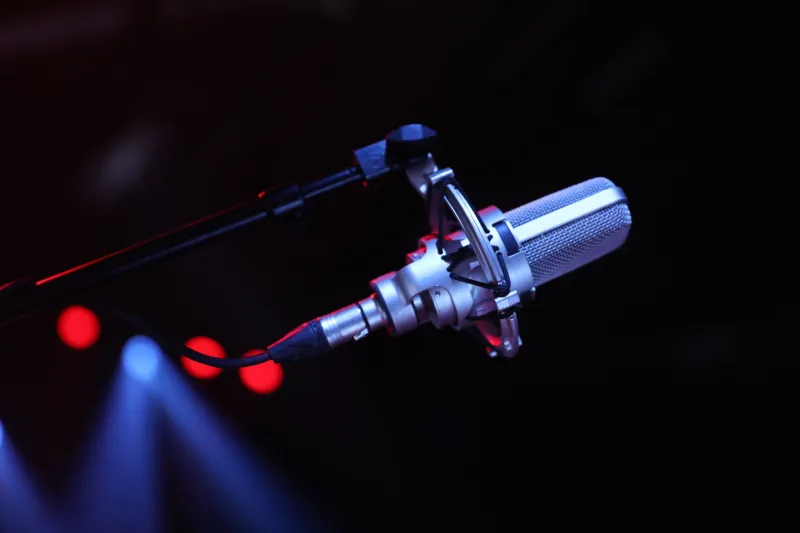
Accurate impulse response acquisition requires attention to the signal chain at every stage. For room measurements, a calibrated measurement microphone—omnidirectional, with a flat response traceable to a known reference—is non-negotiable. Popular choices among US-based acoustic consultants include capsules from Earthworks, DPA, and Brüel & Kjær, typically paired with a low-noise preamplifier and a high-resolution audio interface operating at 48 kHz or 96 kHz sample rates.

The loudspeaker or excitation source should be positioned at the intended listening or performance position, and the microphone placed at representative receiver locations. For room measurements intended to capture reverberation time (RT60 or its variants T20 and T30), multiple microphone positions distributed through the room volume are standard practice, with the final result averaged across positions to reduce spatial variance.

Sweep duration is a critical parameter often underspecified in informal measurements. Longer sweeps increase signal-to-noise ratio but extend measurement time and increase the risk of environmental contamination from HVAC cycling, foot traffic, or outdoor noise. A sweep of six to ten seconds typically provides adequate SNR in reasonably quiet spaces while remaining practical for multi-position surveys.

Windowing Artifacts and How to Avoid Them

Time-domain measurement introduces a complication that frequency-domain work sidesteps: the necessity of windowing. When an impulse response is transformed into the frequency domain for analysis or export, the analyst must decide how much of the time record to include. Truncating too aggressively removes genuine room information; including too much allows noise and late-arriving artifacts to corrupt the result.

For loudspeaker measurements in a reflective environment, a common approach is to apply a time window that captures the direct sound and a short initial period while gating out the first reflection. The reflection-free window available in a given room depends on the geometry: a small treated room might offer only two to three milliseconds before the first boundary reflection arrives, while a large studio control room might provide eight to ten milliseconds. The window boundary should be tapered with a smooth function—a Hann or Tukey window is standard—to avoid the spectral leakage that a hard rectangular truncation would introduce.

The trade-off is frequency resolution. A three-millisecond window limits meaningful frequency-domain resolution to roughly 333 Hz and below, which means that loudspeaker measurements conducted in small rooms with aggressive gating will not accurately represent low-frequency behavior. This is one reason that anechoic chambers or ground-plane outdoor measurements remain the gold standard for full-bandwidth loudspeaker characterization, despite their cost and logistical demands.

Reading the Room: Early Reflections Versus the Reverb Tail

Once a clean impulse response is in hand, the analyst must interpret it. The time record divides naturally into three zones, each carrying distinct information.

The direct sound arrives first and represents the loudspeaker or source radiating without interference. Its amplitude and spectral content reflect the on-axis behavior of the source at the measurement distance.

Early reflections arrive within approximately 80 milliseconds of the direct sound. These are discrete arrivals from nearby boundaries—floor, ceiling, side walls, and rear wall—and they profoundly influence perceived timbre, spatial impression, and speech intelligibility. In a well-designed concert hall, carefully managed early lateral reflections contribute to the sense of envelopment that listeners associate with acoustic richness. In a recording studio control room, strong early reflections from the front wall or console surface create comb filtering artifacts that mislead mixing decisions. Identifying the arrival times of early reflections in the impulse response and tracing them back to specific surfaces is a routine diagnostic step in room treatment design.

The reverb tail follows, comprising the dense, diffuse field of reflections that build up as energy scatters repeatedly through the space. The decay rate of this tail—expressed as RT60, the time required for sound pressure level to fall 60 dB—is the single most cited acoustic metric in architectural standards. ISO 3382 defines measurement procedures for deriving RT60 and related parameters from impulse response data, and US-based projects governed by ANSI standards frequently reference these methods in construction specifications.

A Technique That Earns Its Place

The impulse response measurement workflow is not glamorous. It demands careful setup, disciplined measurement practice, and the interpretive expertise to distinguish meaningful features from artifacts. Yet it consistently delivers information that no frequency-domain specification can replicate. As acoustic simulation tools grow more sophisticated and convolution-based auralizations become routine in design workflows, the measured impulse response has, if anything, grown more central to the profession—not less. Engineers who understand what the time domain is telling them will continue to design spaces and systems that perform as intended, long after the frequency plots have been filed away.