Integration Drift: The Hidden Timing Crisis Threatening Autonomous Vehicle Navigation

At 70 miles per hour on an American interstate, a self-driving vehicle travels roughly 102 feet every second. In that same second, its inertial measurement unit may execute thousands of discrete integration steps, each one accumulating a small but non-trivial timing error into its position estimate. Individually, these errors are inconsequential. Collectively, they define the difference between a vehicle that holds its lane with surgical precision and one that drifts imperceptibly — until it doesn't.
The engineering discipline underlying this problem is not new. Dead reckoning, the practice of estimating current position from a known starting point using velocity and heading data, predates GPS by centuries. What is new is the demand for sub-centimeter accuracy at real-time processing speeds, across a sensor architecture that spans LiDAR, radar, cameras, wheel odometry, and inertial measurement units — each operating on its own internal clock, each contributing its own temporal uncertainty to the fusion pipeline.
The Integration Problem at Its Core
An inertial measurement unit, or IMU, produces measurements of linear acceleration and angular rate at a fixed sampling frequency. To derive position from these measurements, the navigation system performs numerical integration twice: once to convert acceleration into velocity, and again to convert velocity into displacement. Angular rate data undergoes a parallel integration to yield orientation estimates.
The mathematical elegance of this process conceals a fundamental vulnerability. Every integration step is computed using a discrete time interval — a sampling period — that is assumed to be perfectly uniform. In practice, it never is. Clock jitter, interrupt latency, and bus arbitration delays introduce variability into the actual time elapsed between consecutive samples. When the integration algorithm treats these irregular intervals as uniform, it introduces a systematic bias into the position estimate that grows with time.
This is the essence of integration drift: not a single catastrophic error, but the quiet accumulation of many small ones. The drift rate is proportional to the magnitude of the timing uncertainty and the square of the integration duration, meaning that errors compound nonlinearly as a journey extends.
Sensor Fusion and the Timestamping Problem
Modern autonomous vehicle architectures do not rely on IMU data alone. Sensor fusion algorithms — typically variants of the Kalman filter or its nonlinear derivatives — combine IMU outputs with corrections from GPS, LiDAR odometry, visual odometry, and high-definition map matching. The premise is that each sensor type has complementary error characteristics: IMUs drift over time but respond quickly to dynamic changes, while GPS provides absolute position with low drift but at update rates measured in hertz rather than kilohertz.
The fusion architecture introduces a new category of time-domain risk: timestamp misalignment between sensor nodes. A LiDAR unit spinning at 10 Hz and an IMU sampling at 400 Hz are not inherently synchronized. If each sensor applies its own hardware timestamp using a local oscillator, and those oscillators are not disciplined to a common reference, the fusion algorithm will attempt to correlate measurements that do not actually correspond to the same physical moment. The resulting position estimate will reflect a phantom vehicle state — a composite of where the car was at several slightly different instants.
In urban environments at low speeds, this misalignment may produce navigational errors small enough to remain within acceptable tolerances. At highway speeds, the same temporal offset generates lateral position errors that scale directly with vehicle velocity. A 10-millisecond timestamp discrepancy at 70 mph corresponds to approximately 12 inches of position uncertainty — well outside the lane-keeping tolerances that define safe autonomous operation.
Clock Synchronization as a Safety-Critical Discipline
Addressing this problem requires treating clock synchronization not as an infrastructure convenience but as a safety-critical engineering constraint. Several AV platform architectures have adopted IEEE 1588 Precision Time Protocol to distribute a common time reference across all sensor nodes on the vehicle's internal network. PTP enables sub-microsecond synchronization between devices sharing a common Ethernet backbone, substantially reducing the timestamp misalignment that degrades fusion accuracy.
However, PTP introduces its own engineering tradeoffs. The protocol depends on symmetric network propagation delays between the grandmaster clock and each slave node. In automotive environments, network topology, switch latency, and electromagnetic interference can create asymmetric delay paths that corrupt the synchronization offset calculation. Engineers must carefully characterize the vehicle's network architecture to validate that PTP-derived timestamps accurately reflect physical measurement times rather than network-delayed approximations.
An alternative approach used by some developers involves hardware timestamping at the sensor level, where a dedicated timing pulse — often derived from a GPS receiver's pulse-per-second output — triggers a simultaneous timestamp latch across all sensor nodes. This method bypasses software latency entirely but requires careful attention to cable routing, signal integrity, and the propagation delay of the timing pulse itself across the vehicle's physical architecture.
Update Rate, Latency, and the Computational Tradeoff
Increasing IMU sampling frequency is an intuitive response to integration drift: finer time resolution reduces the interval over which timing errors accumulate. But higher update rates impose proportionally greater demands on the computational pipeline. A sensor fusion algorithm processing 1,000 IMU samples per second must complete its state estimation within one millisecond to remain current — a constraint that becomes increasingly difficult to satisfy as the complexity of the fusion model grows.
This creates a practical tension between temporal fidelity and computational latency. An algorithm that achieves perfect timestamping accuracy but requires 50 milliseconds to complete its state update will still produce a stale position estimate by the time it reaches the vehicle's control systems. At highway speeds, 50 milliseconds of algorithmic latency corresponds to more than five feet of vehicle travel — a distance over which road conditions, lane curvature, and surrounding traffic can change meaningfully.
AV engineers navigate this tradeoff through a combination of hardware acceleration, predictive state extrapolation, and tiered fusion architectures that separate high-rate IMU propagation from lower-rate absolute correction updates. The IMU integration loop runs at full sampling frequency on dedicated hardware, while GPS and LiDAR corrections are applied asynchronously as they become available. The accuracy of this architecture depends critically on the precision with which each correction is time-tagged and applied at the correct point in the integration history.
Error Propagation Models and Validation
Characterizing integration drift requires rigorous error propagation modeling that accounts for IMU noise density, bias instability, and clock uncertainty simultaneously. The Allan deviation, a tool long established in precision timing and oscillator characterization, has found application in IMU performance analysis precisely because it decomposes error contributions across different averaging intervals — revealing whether a system's dominant error source is white noise, bias drift, or rate random walk.
Validation of these models in the context of autonomous vehicles demands test environments that can expose the system to the full range of dynamic conditions it will encounter in deployment: sustained highway cruising, urban stop-and-go traffic, highway on-ramp acceleration, and emergency braking. Each scenario exercises a different portion of the IMU's dynamic range and a different regime of the integration error accumulation curve.
For AV developers, this validation process is not merely an engineering exercise. It is the empirical foundation upon which safety cases are built and regulatory submissions are grounded. As the National Highway Traffic Safety Administration continues to develop its framework for autonomous vehicle certification, the ability to demonstrate quantified bounds on navigation uncertainty — including the time-domain error contributions of integration drift — will become an increasingly central element of the approval process.
The physics of dead reckoning have not changed. What has changed is the consequence of getting it wrong.