Temporal Coincidence Is Not Causation: Breaking the Correlation Trap in Transient Fault Diagnosis

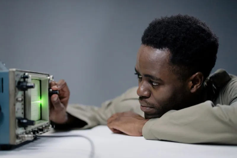
There is a particular kind of confidence that comes from watching two waveforms converge on an oscilloscope screen. The spike in current appears. A half-millisecond later, the vibration sensor fires. The engineer notes the sequence, draws an arrow on the printout, and writes "root cause identified" in the incident log. It feels rigorous. It is not.

The misidentification of correlated transients as causally linked events is one of the most persistent analytical errors in time-domain engineering. It costs organizations in unnecessary component replacements, extended downtime, and — in safety-critical applications — genuine hazard. Understanding why it happens, and how to prevent it, requires a clear-eyed look at both the physics of signal propagation and the cognitive shortcuts that experienced engineers are just as susceptible to as novices.

Why the Brain Wants a Story

Human cognition is tuned for narrative. When two events occur in close temporal proximity, the mind constructs a causal link almost automatically. This tendency — well-documented in cognitive psychology — is amplified in control room environments where engineers are under pressure to identify faults quickly and restore operation. The time-domain display, with its crisp visual representation of event sequences, feeds directly into this instinct.

The problem is that physical systems are densely interconnected. In a typical industrial drive train, a single mechanical fault will simultaneously disturb current draw, shaft vibration, bearing temperature gradients, and acoustic emission — often within a window of tens of milliseconds. Every one of those signals will appear to "follow" every other. Cross-correlation functions will show strong peaks. Lag values will be nonzero but small. The data looks exactly like causation. It is, in most cases, co-effect.

The Shared-Excitation Problem

Consider a case that illustrates the pattern cleanly. A mid-sized manufacturing facility in the Ohio River Valley was experiencing repeated failures in a variable-frequency drive controlling a pump motor. Engineers captured time-domain data showing that voltage transients on the DC bus consistently preceded anomalous current spikes in the motor windings by approximately 800 microseconds. The diagnosis: bus voltage instability was inducing overcurrent events. The fix: a new line reactor and additional bus capacitance. The failures continued.

Subsequent analysis — conducted after a third replacement cycle — revealed that both the bus transient and the current spike were downstream effects of a common cause: intermittent contact resistance in a connector on the motor feedback cable. The feedback dropout caused the drive controller to issue a rapid torque command correction, which simultaneously perturbed the DC bus and demanded excess current from the inverter stage. The 800-microsecond lag between the two observed signals reflected nothing more than the different propagation paths from a single upstream disturbance to two different measurement points.

The engineers had not been careless. They had been systematic. But their system lacked a critical step: validation of the proposed causal chain against a physical model of the mechanism.

Propagation Delay as a Red Herring

One of the subtler contributors to causal misattribution is the presence of genuine, measurable time delays between signals. Engineers are trained to interpret lag as directional information — signal A leads signal B, therefore A influences B. In many well-behaved linear systems, this reasoning is sound. In nonlinear, multi-path physical systems, it is frequently misleading.

Consider electromagnetic interference in a mixed-signal test environment. A switching power supply generates a burst of high-frequency noise. That noise couples into a sensor cable through electric field induction and also propagates through the ground plane to the ADC reference input. Depending on cable routing and board layout, the two coupled artifacts may arrive at the measurement system with a relative delay of several hundred nanoseconds to a few microseconds. A cross-correlation analysis will identify a strong peak at that lag and suggest that one interference path is driving the other. Neither is driving the other. Both are driven by the supply.

The delay is real. The causal interpretation is wrong.

Establishing the Causal Chain: A Practical Framework

Rigorously distinguishing causation from correlation in transient analysis requires moving beyond the waveform display into physical mechanism validation. A useful framework involves three sequential tests.

Mechanism plausibility. Before interpreting a time-lag relationship as causal, the analyst should articulate the specific physical mechanism by which signal A could produce signal B. This mechanism must be consistent with known system physics, including propagation velocities, transfer function bandwidths, and energy constraints. If no plausible mechanism exists, the correlation is a flag for shared excitation, not a causal link.

Intervention testing. Where possible, the hypothesized cause should be independently stimulated while the proposed effect is monitored. If injecting the cause-signal artificially — through a function generator, a controlled fault insertion, or a calibrated disturbance — does not reproduce the effect, the causal hypothesis is weakened substantially. This is the closest analog available in field engineering to a controlled experiment.

Residual signal analysis. After subtracting the contribution of the hypothesized cause from the observed effect signal, engineers should examine the residual. A genuine causal relationship will produce a residual that approaches measurement noise. A spurious correlation will leave a structured residual that reflects the true shared excitation source.

The Granger Trap in Engineering Practice

Some engineers familiar with time-series analysis will reach for Granger causality testing as a formal tool. Granger causality, developed originally for econometric forecasting, asks whether the past values of signal A improve predictions of signal B beyond what B's own history provides. It is a statistically defensible concept that has migrated into engineering signal analysis, particularly in condition monitoring applications.

The limitation is fundamental: Granger causality is a predictive concept, not a physical one. A signal can be Granger-causal for another without any direct physical link between them, provided both are driven by a common process with differential delays. In systems where shared excitation sources are common — which describes virtually every multi-sensor industrial installation — Granger analysis can systematically endorse spurious causal hypotheses.

Used alongside physical mechanism validation, Granger testing is a useful screening tool. Used in isolation, it reproduces the same correlation trap with additional mathematical credibility.

Toward Disciplined Transient Analysis

The solution is not skepticism about time-domain data. The waveform record remains one of the most information-dense diagnostic tools available to the practicing engineer. The solution is a disciplined separation between observation and interpretation.

Observation establishes what signals appeared, when, in what sequence, and with what morphology. Interpretation assigns physical meaning to those observations. The gap between the two is where causal errors are born. Closing that gap requires explicit mechanism hypotheses, wherever possible validated through intervention, and a standing willingness to consider shared excitation as the default explanation when multiple signals respond simultaneously to a system disturbance.

The correlation peak on the cross-correlation plot is a starting point for analysis. It is never, by itself, a diagnosis.