Blind Spots in the Data: How Undersampling Is Quietly Sabotaging Industrial Monitoring Systems

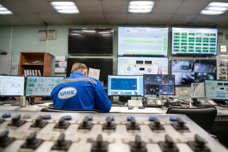
There is a particular category of engineering failure that receives far less attention than it deserves: the failure to observe. Unlike a sensor that returns an erroneous value or a communication link that drops packets, an undersampled acquisition system presents its data with complete confidence. The timestamps are clean, the waveforms appear continuous, and the trending dashboards update on schedule. What the system does not show—and cannot show—are the events it was never fast enough to capture.

This is the aliasing problem, and in 2024, it is embedded far more deeply into American industrial monitoring infrastructure than most engineers would care to acknowledge.

The Nyquist Boundary and What Happens When You Cross It

Claude Shannon's sampling theorem establishes an unambiguous requirement: to faithfully reconstruct a signal, the sampling rate must exceed twice the highest frequency component present in that signal. This threshold—the Nyquist frequency—is not a guideline or a rule of thumb. It is a mathematical boundary. Cross it, and the acquisition system begins misrepresenting reality in a specific and insidious way: high-frequency content folds back into the recorded spectrum, masquerading as lower-frequency phenomena.

In a laboratory setting, aliasing is a textbook concept that engineers understand and deliberately avoid. In deployed industrial systems, however, the conditions that produce aliasing accumulate gradually and often without formal review. A monitoring system installed for one purpose gets repurposed for another. Sampling rates chosen for steady-state observation get applied to transient detection. Anti-aliasing filters specified for one sensor bandwidth get paired with replacement sensors carrying wider frequency responses. The result is a monitoring architecture that was never designed for what it is currently being asked to do.

Vibration Monitoring: Where the Problem Is Most Severe

Rotating machinery is among the most demanding environments for time-domain acquisition, and it is also where undersampling causes the most consequential blind spots. Bearing defect frequencies, for instance, are calculated from shaft speed and geometric constants, and they can extend into ranges well above what many permanently installed vibration monitoring systems are configured to capture.

Consider a common scenario: a plant engineer installs a continuous vibration monitoring system on a high-speed compressor. The system samples at 1 kHz, which appears reasonable for general vibration trending. What that rate cannot capture are the impulsive events associated with early-stage bearing raceway defects, which may contain significant energy at 3 to 5 kHz or higher depending on the machine's operating speed. The monitoring system records smooth, unremarkable vibration data right up until the bearing fails catastrophically. A post-incident review of the acquisition records reveals nothing actionable, because the diagnostic information was never acquired in the first place.

This scenario is not hypothetical. It is a recurring pattern in post-failure analyses across petrochemical, paper, and food processing facilities throughout the United States.

Power Quality: Transients That Disappear Before the Recorder Sees Them

Power quality monitoring presents a different but equally serious manifestation of the aliasing problem. Voltage transients caused by switching events, capacitor bank operations, or lightning-induced surges can have rise times measured in microseconds. A power quality analyzer sampling at 256 samples per cycle—a common configuration for harmonic analysis—operates at roughly 15.36 kHz at 60 Hz fundamental. That rate is entirely appropriate for harmonic content up to the seventh or ninth order, but it is categorically insufficient for capturing high-frequency transients.

The practical consequence is that equipment damage events and nuisance trips attributable to transient overvoltages frequently occur without any corresponding record in the power quality monitoring system. Maintenance engineers are left investigating equipment failures with no timestamp evidence, no waveform data, and no basis for distinguishing between a transient fault and an insulation degradation problem. The monitoring system has not failed in any conventional sense. It has simply been operating outside its valid frequency range without anyone recognizing the mismatch.

A Framework for Auditing Existing Acquisition Systems

Correcting an undersampling problem in a deployed monitoring system requires a structured approach that begins with characterizing the signals being monitored rather than the equipment doing the monitoring.

Step one: Establish the true frequency content of each monitored signal. This requires either theoretical analysis based on known physics—bearing defect frequency calculations, switching transient rise time estimates, motor current harmonic structure—or a short-duration high-bandwidth reference measurement using calibrated instrumentation. The goal is to determine the highest frequency component that carries diagnostic relevance, not merely the highest frequency present.

Step two: Verify anti-aliasing filter cutoff frequencies. Many installed monitoring systems include analog anti-aliasing filters, but filter specifications are often not documented at the system level. A filter with a cutoff frequency above the Nyquist limit of the digitizer provides no protection against aliasing. Confirm that the filter's roll-off is sufficient to attenuate all signal content above the Nyquist frequency before digitization occurs.

Step three: Apply a conservative sampling margin. The Nyquist criterion defines a theoretical minimum. Practical systems should target a sampling rate of five to ten times the highest frequency of interest, not two times. This margin accommodates filter transition bands, accounts for signal content that was not anticipated during system design, and preserves temporal resolution for accurate event timestamping.

Step four: Audit data reduction stages. Many industrial monitoring platforms apply decimation or averaging after initial acquisition, reducing the effective sample rate stored to disk or transmitted over the network. Engineers who specify the front-end sampling rate correctly may still lose high-frequency content if downstream data reduction is applied without appropriate pre-filtering.

Step five: Validate with known test signals. Before relying on an audited system for critical monitoring, inject a test signal at the highest frequency of interest and confirm that the acquisition chain captures it faithfully. This step catches configuration errors, firmware limitations, and hardware bandwidth constraints that may not appear in system documentation.

Calculating Safe Sampling Rates Before Deployment

For new monitoring deployments, the sampling rate calculation should be treated as a formal design step rather than a default selection. Begin with the application's diagnostic requirements. For rolling element bearing monitoring, calculate the ball pass frequency outer race (BPFO) and ball pass frequency inner race (BPFI) at maximum operating speed, then multiply by the number of harmonics required for reliable detection—typically five to ten. For power quality transient capture, reference IEEE Standard 1159, which provides guidance on measurement bandwidth requirements for different transient categories.

Once the required bandwidth is established, select a digitizer with a sample rate at least five times that bandwidth, confirm that the anti-aliasing filter cutoff falls below the Nyquist frequency with adequate attenuation slope, and document both parameters in the system specification. This documentation step is not bureaucratic formality. It is the record that allows future engineers to evaluate whether the system remains appropriate as operating conditions evolve.

The Cost of Assuming Completeness

The aliasing epidemic in industrial monitoring is sustained by a reasonable but incorrect assumption: that a system generating continuous data is a system capturing complete information. The Nyquist theorem defines the precise conditions under which that assumption holds, and those conditions are violated routinely in deployed infrastructure.

For engineers responsible for monitoring systems—whether in manufacturing, utilities, or process industries—the appropriate response is not alarm but audit. The framework described above is not complex. It requires time and access to system documentation, but it does not require new hardware in most cases. What it requires is a willingness to question whether the data a monitoring system is producing is actually the data the application demands.

In time-domain signal acquisition, the events you miss are indistinguishable from the events that never occurred. That distinction matters enormously when the next maintenance decision, or the next equipment failure, depends on the integrity of the record.